Examples
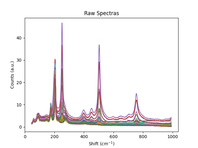
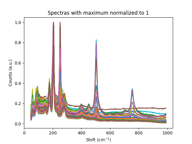
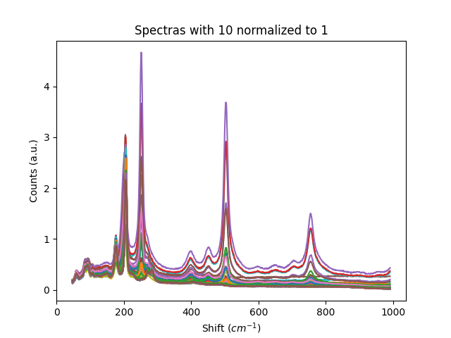
Example 1: Normalization methods
"""
This example shows some of the normalization functions available.
"""

# import the library
import spectrapepper as spep

# load data
x, y = spep.load_spectras()

# normalize each spectra to its maximum value
norm1 = spep.normtomax(y)

# normalize to 10, that is, 10 will become 1.
norm2 = spep.normtovalue(y, val=10)

# normalize to the global maximum of all the data
norm3 = spep.normtoglobalmax(y)

# visualization
import matplotlib.pyplot as plt

sets = [y, norm1, norm2, norm3]
titles = ['Raw Spectras', 'Spectras with maximum normalized to 1', 'Spectras with 10 normalized to 1',
          'Spectras with global maximum normalized to 1']

for i,j in zip(sets, titles):
    for k in i:
        plt.plot(x, k)
    plt.title(j)
    plt.xlabel('Shift ($cm^{-1}$)')
    plt.ylabel('Counts (a.u.)')
    plt.show()
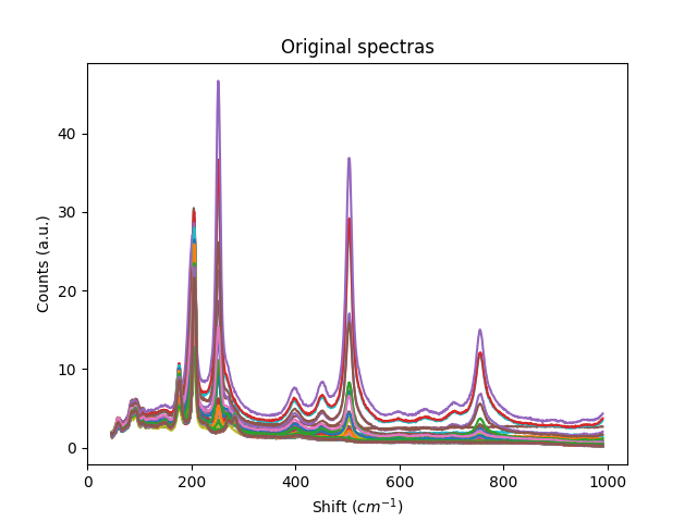
Example 2: Spectral pre-processing
"""
This example shows simple processing of Raman spectras.
"""
# import the library
import spectrapepper as spep
# load data
x, y = spep.load_spectras()
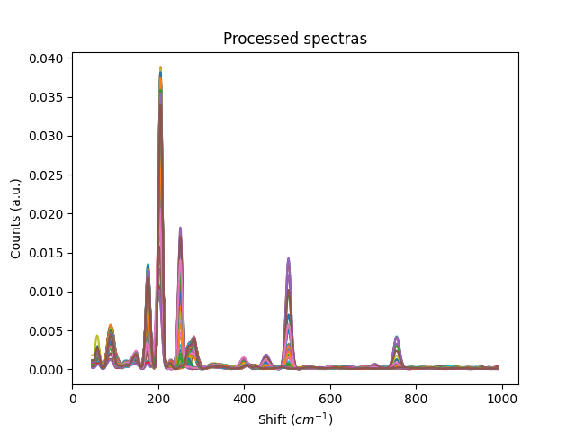
# remove baseline
newdata = spep.alsbaseline(y)
# remove noise with moving average
newdata = spep.moveavg(newdata, 5)
# norm the sum to 1
newdata = spep.normsum(newdata)
# visualization
import matplotlib.pyplot as plt
for i in y:
plt.plot(x, i)
plt.title('Original spectras')
plt.xlabel('Shift ($cm^{-1}$)')
plt.ylabel('Counts (a.u.)')
plt.show()
for i in newdata:
plt.plot(x, i)
plt.title('Processed spectras')
plt.xlabel('Shift ($cm^{-1}$)')
plt.ylabel('Counts (a.u.)')
plt.show()
Example 3: Pearson, Spearman, and Grau analyses
"""
This example shows how to use pearson and spearman matrices and grau plot.
"""

# import the library
import spectrapepper as spep

# load data
data = spep.load_params()

# labels
labels = ['T', 'A1', 'A2', 'A3', 'A4', 'A5', 'S1', 'R1', 'R2', 'ETA', 'FF', 'JSC', 'ISC', 'VOC']

# plot spearman
spep.spearman(data, labels)

# plot pearson
spep.pearson(data, labels)

# plot grau.
spep.grau(data, labels)
Example 4: Machine learning preparation
"""
This example shows how to use Scikit-learn for spectral data with spectrapepper.
"""

# import libraries
import spectrapepper as spep

# load data
x, y = spep.load_spectras()

# load targets
targets = spep.load_targets()

# shuffle data
features, targets = spep.shuffle([y, targets], delratio=0.1)

# target classification
classtargets, labels = spep.classify(targets, glimits=[1.05, 1.15], gnumber=0)

# machine learning
from sklearn.discriminant_analysis import LinearDiscriminantAnalysis
import pandas as pd

lda = LinearDiscriminantAnalysis(n_components=2)
LDs = lda.fit(features, classtargets).transform(features)
df1 = pd.DataFrame(data=LDs, columns=['D1', 'D2'])
df2 = pd.DataFrame(data=classtargets, columns=['T'])
final = pd.concat([df1, df2], axis=1)
prediction = lda.predict(features)

# visualization
spep.plot2dml(final, labels=labels, title='LDA', xax='D1', yax='D2')
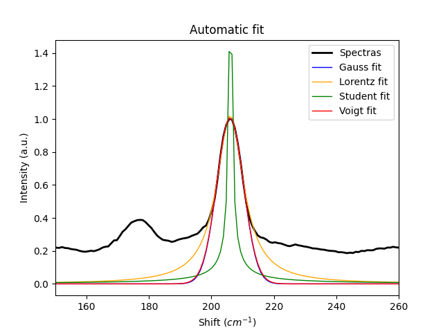
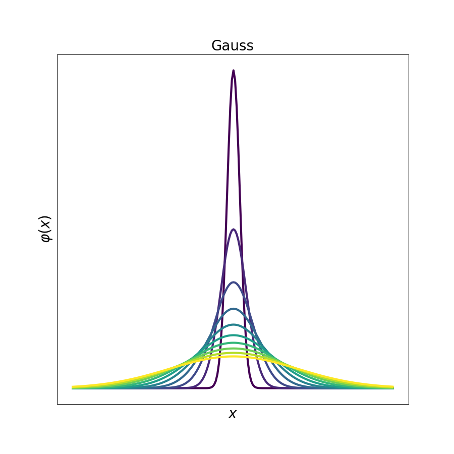
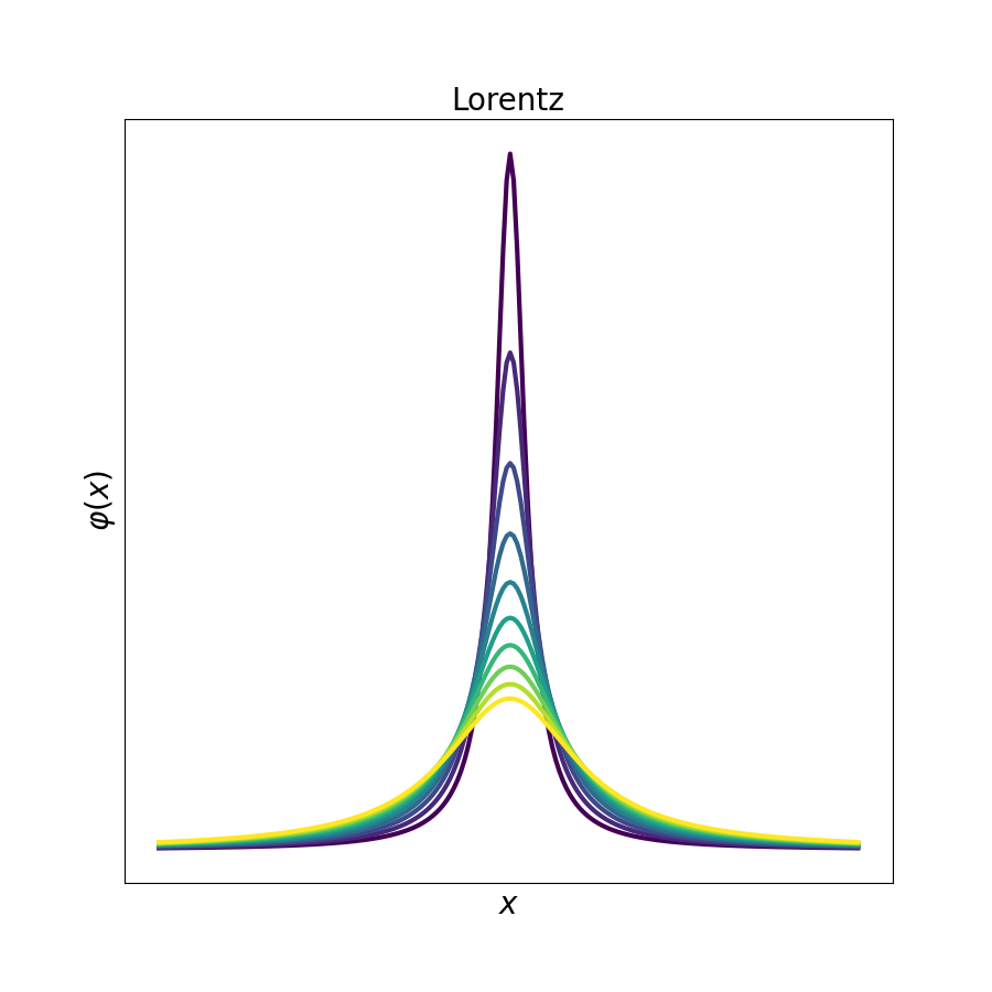
Example 5: Curve fittings
"""
This example shows how to use different distribution fittings on experimental
spectroscopic data. Student distribution is shown just as example, but it is
not suitable for the particular peak tested. It is also important to notice
that the fit greatly depends on the resolution of the curve. If needed,
it is possible to first extrapolate to a greater resolution.
"""
# import libraries
import spectrapepper as spep
import matplotlib.pyplot as plt
# load data to fit
x, y = spep.load_spectras(sample=10) # load 1 single spectra from the data
y = spep.normtomax(y) # Normalize the maximum value to 1
# select peak to fit to
peak = 206 # approximate position of the peak (in cm-1) to be evaluated
# automatically fit the distributions to the peak in the data
gauss = spep.gaussfit(y=y, x=x, pos=peak, look=5)
lorentz = spep.lorentzfit(y=y, x=x, pos=peak, look=5)
student = spep.studentfit(y=y, x=x, pos=peak, look=5)
voigt = spep.voigtfit(y=y, x=x, pos=peak, look=5)
curves = [y, gauss, lorentz, student, voigt]
labels = ['Spectras', 'Gauss fit', 'Lorentz fit', 'Student fit', 'Voigt fit']
colors = ['black', 'blue', 'orange', 'green', 'red']
linewd = [2, 1, 1, 1, 1]
for curve, label, color, linew in zip(curves, labels, colors, linewd):
plt.plot(x, curve, label=label, lw=linew, c=color)
plt.xlim(150, 260)
plt.xlabel('Shift ($cm^{-1}$)')
plt.ylabel('Intensity (a.u.)')
plt.title('Automatic fit')
plt.legend()
plt.show()
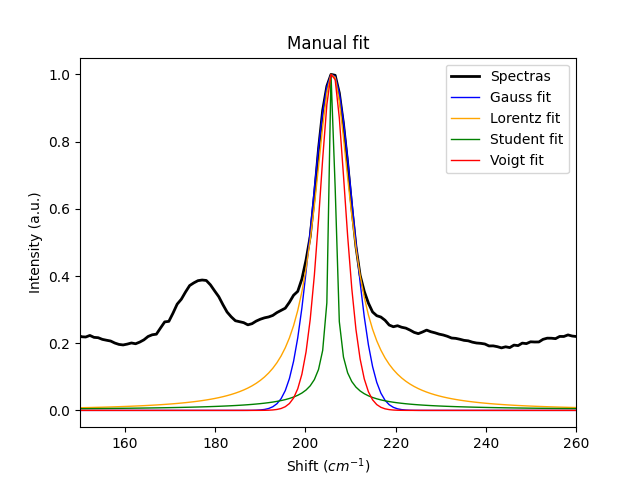
# manually fit the distributions to the peak.
gauss = spep.gaussfit(y=y, x=x, pos=peak, sigma=4.4, manual=True)
lorentz = spep.lorentzfit(y=y, x=x, pos=peak, gamma=5, manual=True)
student = spep.studentfit(y=y, x=x, pos=peak, v=0.1, manual=True)
voigt = spep.voigtfit(y=y, x=x, pos=peak, sigma=4.4, gamma=5, manual=True)
curves = [y, gauss, lorentz, student, voigt]
for curve, label, color, linew in zip(curves, labels, colors, linewd):
plt.plot(x, spep.normtomax(curve), label=label, lw=linew, c=color)
plt.xlim(150, 260)
plt.xlabel('Shift ($cm^{-1}$)')
plt.ylabel('Intensity (a.u.)')
plt.title('Manual fit')
plt.legend()
plt.show()
# show how the distribution changes by the change in the parameters
gauss,lorentz, student, voigt = [], [], [], []
for i in range(10):
gauss.append(spep.gaussfit(sigma=4*(i+1), manual=True))
lorentz.append(spep.lorentzfit(gamma=(5+i*2), manual=True))
student.append(spep.studentfit(v=0.1*(1+1*i), manual=True))
voigt.append(spep.voigtfit(gamma=(5+i*3), sigma=4*(i+3), manual=True))
# the stackplot fuinction is a nice tool to show the evolution of data
for i, j in zip([gauss, lorentz, student, voigt], ['Gauss', 'Lorentz', 'Student', 'Voigt']):
spep.stackplot(i, offset=0, lw=3, figsize=(9, 9), xlabel='$x$',
ylabel=r'$\varphi (x)$', cmap='viridis', title=j)
Example 6: Spectroscopic data set macro analysis
"""
This example shows basic analysis of a set of spectras.
"""

import spectrapepper as spep

# load data set
x, y = spep.load_spectras()

# remove baseline
y = spep.bspbaseline(y, x, points=[158, 243, 315, 450, 530], plot=False)

exit()

# Normalize the spectra to the maximum value.
y = spep.normtoratio(y, r1=[190, 220], r2=[165, 190], x=x)

# Calculate the averge spectra of the set.
avg = spep.avg(y)

# Calculate the median spectra of the set. That is, a synthetic spectra
# composed by the median value in each wavenumber.
med = spep.median(y)

# Calculate the standard deviation for each wavenumber.
sdv = spep.sdev(y)

# Obtain the typical sample of the set. That is, the spectra that is closer
# to the average.
typ = spep.typical(y)

# Look for the representative spectra. In other words, the spectra that is
# closest to the median.
rep = spep.representative(y)

# Calculate the minimum and maximum spectra. That is, the minimum and maximum
# values for each wavenumber. They are calculated together.
mis, mas = spep.minmax(y)

# visualiz the results
import matplotlib.pyplot as plt

curves = [avg, med, sdv, typ, rep, mis, mas]
titles = ['Average', 'Median', 'St. Dev.', 'Typical',
          'Representative', 'Minimum', 'Maximum']

for i in y:
    plt.plot(x, i, lw=0.5, alpha=0.2, c='black')
for i,j in zip(curves, titles):
    plt.plot(x, i, label=j)
plt.legend()
plt.ylabel('Intensity (a.u.)')
plt.xlabel('Shift ($cm^{-1}$)')
plt.xlim(100, 600)
plt.ylim(-0.3, 0.9)
plt.show()
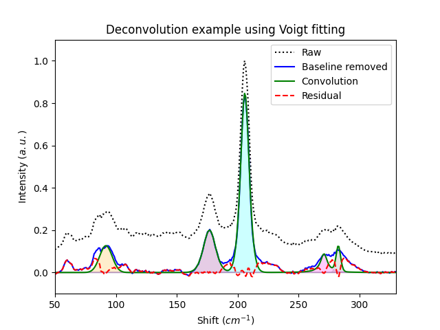
Example 7: Deconvolution of a spectra
"""
This examples shows an application of a manual and self-resolved
deconvolution with Voigt fittings of some of the peaks shown in the
spectra.
"""
import spectrapepper as spep
import matplotlib.pyplot as plt
import numpy as np

# load data
x, y = spep.load_spectras(1)
y = spep.normtomax(y)

# some processing
y_b = spep.bspbaseline(y, x, points=[155, 243, 315, 450, 530])

# define peak positions and fitting ranges
positions = [95, 175, 205, 270, 285]
ranges = [4, 10, 10, 2, 2]

# calculate and save the fittings
fittings = []
for i in range(len(positions)):
    temp = spep.voigtfit(y_b, x, pos=positions[i], look=ranges[i])
    fittings.append(temp)

# residual and fitting convolution
residual = np.array(y_b)
convolution = [0 for _ in y]
for i in fittings:
    residual -= i
    convolution += i

# plot of all the fittings
colors = ['orange', 'purple', 'cyan', 'magenta', 'grey']
for curve, color in zip(fittings, colors):
    plt.fill_between(x, curve, 0, color=color, alpha=0.2)

# plot all the other things
curves = [y, y_b, convolution, residual]
colors = ['black', 'blue', 'green', 'red']
lineseg = [':', '-', '-', '--']
labels = ['Raw','Baseline removed', 'Convolution','Residual']

for curve, color, line, label in zip(curves, colors, lineseg, labels):
    plt.plot(x, curve, c=color, ls=line, label=label)

plt.title('Deconvolution example using Voigt fitting')
plt.xlabel('Shift ($cm^{-1}$)')
plt.ylabel('Intensity ($a.u.$)')
plt.xlim(50, 330)
plt.ylim(-0.1, 1.1)
plt.legend()
plt.show()